-
What We Do
-
AI NavigatorGain clear direction and momentum as your chart your organization’s AI path.
-
AI FoundationsEstablish the essential skills, systems, and mindset to support sustainable AI adoption.
-
Agentic AI LabExplore, prototype, and refine agent-driven solutions to accelerate real-world impact.
-
GovLabAdvance government innovation with practice AI solutions tailored to unique public sector needs.
-
-
Featured
 The AI Agent Advantage: Understanding Your Digital Workforce
-
Some Industries We Support
-
Featured
 Building Canadian Communities with Homegrown AI


Insights
Understanding Security Sensitivity to Good and Bad Times Through Mixture Models

We explore how to leverage Gaussian Mixture Models (GMM) to model regime dependent betas
While investors have often suspected that a security’s price sensitivity to the overall market varies across time, and can change dramatically during periods of market turmoil, it’s not entirely clear how to measure this phenomenon.
One approach taken is to divide up our historical sample of security prices, and subjectively judge which periods we believe represent the regimes of interest (e.g. periods of low vs high market volatility, periods of market drawdowns, etc).
While this approach can be useful, its main drawback is how it relies on our subjective assessments of what represented historically a “good” or “bad” period for the market.
In this article, we’ll instead turn to an alternative approach that relies on statistically modelling the processes underlying the security in question (and the market as a whole) as Gaussian mixtures.
Gaussian Mixture Models
The Gaussian in the name refers to the academic name applied to the so-called Bell-curve, or “Normal,” distribution we’re all familiar with.
A Gaussian mixture is therefore a mixture of Bell-curve distributions.
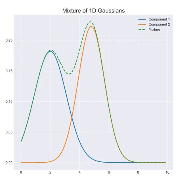
A mixture of two Gaussian distributions.
It turns out that mixing Bell-curve distributions has the desirable property that it can well represent the distribution of a security (or the market’s) price returns, that aren’t themselves actually Normally distributed.
Moreover, using such a mixture can help us identify when a security’s return was generated during either a “good” or “bad” regime.1
Essentially we want to use the Gaussian mixture model (herein GMM) to discover the security’s return distributions for both the “good” and “bad” states of the market.
We then want to determine the sensitivity of the security’s price returns to the market as a whole during these “good” and “bad” states, in comparing them.
This sensitivity is usually measured as Beta, and we will maintain that convention here as well. Therefore, the GMM model facilitates comparison of the security’s measured Beta during the “good” and “bad” states automatically.
Finally, we can use the GMM model to determine which state the security’s price was in, historically.
In this sense, the GMM can be considered a “regime model.”
Example Setup – GMM on Barrick Gold
For this particular example, we will use the market’s current, and lagged returns, as the inputs that determine the regime state at any time ‘t’.
- Our proxy for the market will be the SPDR S&P500 ETF (ticker: SPY).
- The target security for the model is chosen as Barrick Gold (ticker: GOLD).
Why Barrick Gold?
- Barrick Gold is chosen as an example here, given the oft-cited expectation that its Beta is roughly zero.
- The story goes, that Barrick Gold, being a gold mining company, shouldn’t in principle be affected by what happens in the equity markets.
- We will show that during periods of market crisis, the Beta on Barrick Gold stock can change dramatically.