A Random Walk Down the Factor Zoo

We explore how leveraging simulated random factors can improve statistical rigor around factor-based quant strategies

A blindfolded monkey throwing darts at a newspaper’s financial pages could select a portfolio that would do just as well as one carefully selected by experts.

Since the 1990’s, factor-based quant strategies have continued to increase in popularity.

The standard style factors, such as size, value, momentum, growth, beta, etc, have all become widely known, and investment practitioners have employed them in their own variations of factor portfolio-based strategies.

That said, the dissemination of the so-called “factor zoo” has not come without its own set of issues.

For one, given the wide variety of factors popularized in both academia as well as the sell-side literature, it’s hard to know which factors to invest in. 

Often investors rely on historical backtests of factor performance.

But given the large number of factors and their variations, could it be that what looks like a significant historical backtest may have simply been due to random chance? 

After all, if we try enough random permutations of factors and their variations, we may find what looks to be a legitimate signal, but that this signal performs poorly out-of-sample into the future.

At AlphaLayer, we strive to build strategies with a high level of statistical rigor and while a backtest may look good it is only real-world performance that matters.

So how can we better understand factor significance? And as a result, increase the probability of delivering better factor-based strategies?

Random Factor Simulations

One of the ways we look to better understand the statistical significance of factor portfolios is by leveraging random simulations.

That is, we ask ourselves questions like:

• If we were to randomly choose stocks in a factor portfolio, based on random factor loadings that look “similar enough” to real factor loadings, what kind of performance would we expect to observe in these factor portfolios, on average?  
• Moreover, what would we expect a factor research program, based on skilled stock selection, to look like, versus one no different than choosing at random?

In other words, instead of having a monkey throw darts at a financial newspaper, we get a monkey to throw darts at factor loadings.

Approach to Random Factor Simulation

As a simple example, let’s take the S&P 500 universe, where we allow our factor portfolios to take on positions, historically, if those securities were within the S&P 500 index on that date.

Subsequently each day, we randomly generate fake factor loadings for each security in our universe, each drawn from the Gaussian distribution with a mean of 0 and standard deviation of 1. 

Loadings also follow a time-series stochastic process that exhibits lag 1 serial autocorrelation (i.e. an AR(1) process) with a coefficient of persistence set to 0.90. 

That is, the value of the factor loading for any given security, from one day to the next is always:

This is designed to simulate the often-observed phenomenon of slowly changing factor loadings.

Next, we z-score these loadings each day in the cross-section of securities and convert the loadings to long/short neutral portfolio weights.

We then run a historical backtest using these weights and record a number of performance metrics, including the historical daily return, annualized Sharpe Ratio (SR).

Now, we repeat the above steps 100 times, each time performing a historical backtest. In the first chart below we plot what we get in terms of historical cumulative returns to the 100 different factor portfolios:

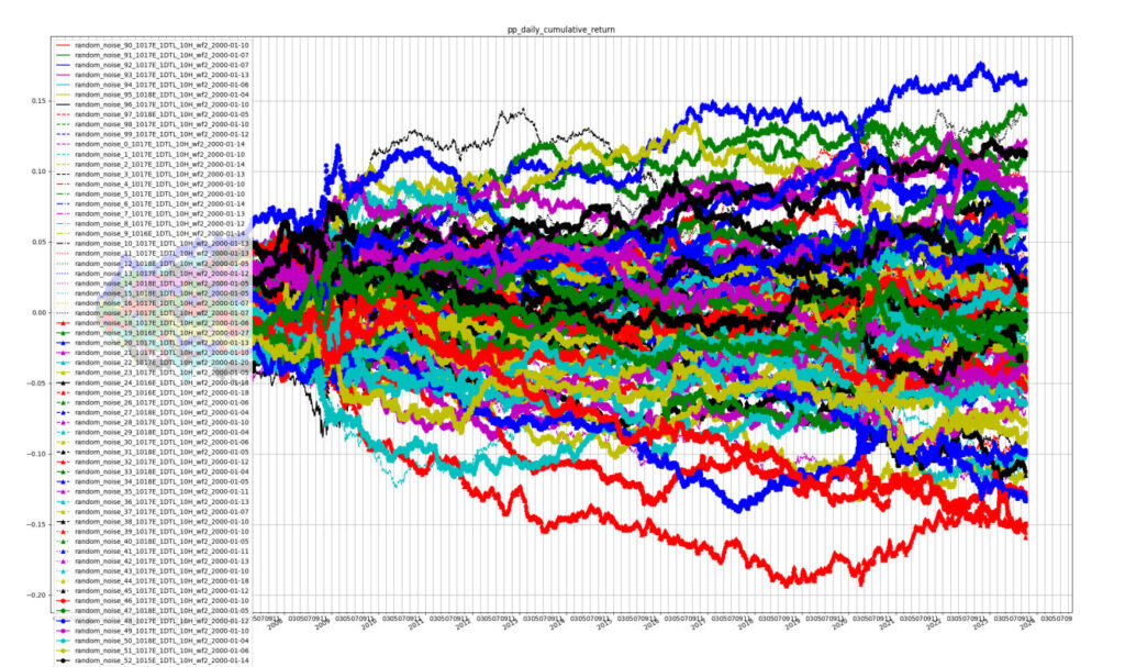
Cumulative returns to random noise factor portfolios.

Moreover, the chart below displays the distribution of the annualized SR values for each cumulative return series above:

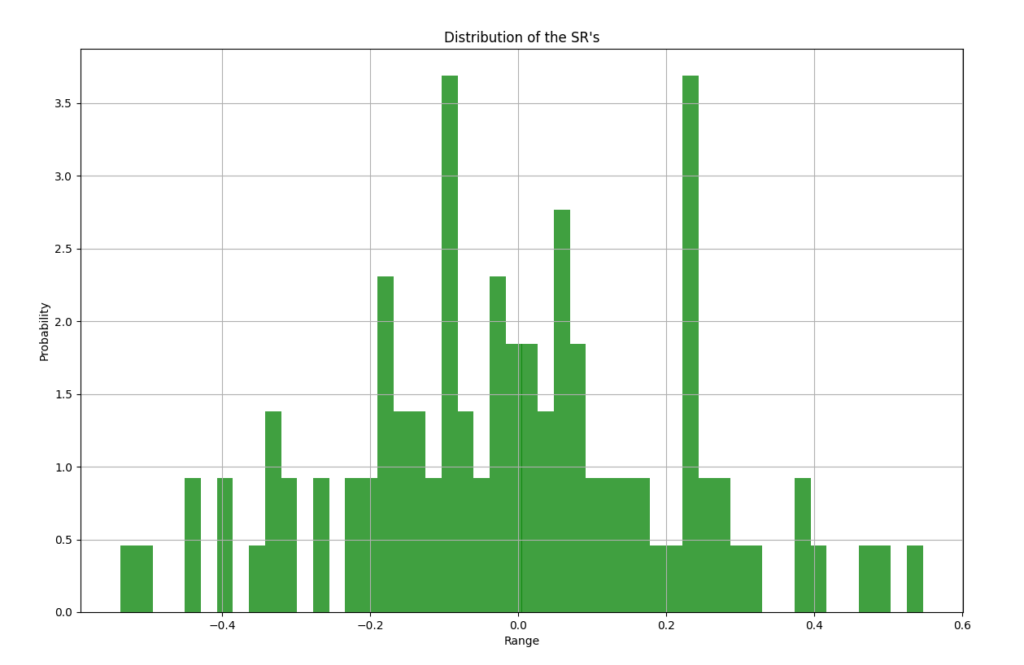
SR distribution from random factor portfolios.

We can then use these SR values to compute the 95% confidence intervals of observing the SR from this random noise distribution.

Computing both the 2.5% and 97.5% quantiles of the SR distribution, we find the values [-0.438726, 0.439018] or roughly [-0.44, 0.44].

That is, 95% of the SR values we observed during simulations of random noise factor portfolios, fell within this range.

Finally, we can use the SR distribution to estimate the empirical CDF function (ECDF). The ECDF estimates the probability of observing a SR less than the given value, for each value observed.  The estimated ECDF function is plotted below:

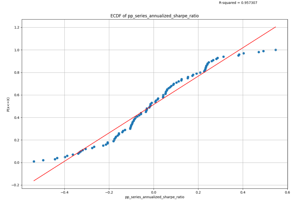
ECDF of SR distribution.

So, for example, the probability of seeing a SR less than roughly 0.55 is 100%, at least in our sample, since we never observed a random factor portfolio with an SR greater than this.

It’s worth noting that if we increased the number of random simulations to be larger than 100, the distribution of the SRs would become more well-defined and would eventually take on a “bell-curve” Gaussian shape as the number of simulations grows.

Real-world Application

Suppose now that we build a factor portfolio with real data, and we observe performance that doesn’t exceed the 95% confidence intervals of our random results above (i.e. we observe an SR less than 0.44 in absolute value). 

This certainly doesn’t imply that the factor is illegitimate, but it does suggest it’s possible these real-world results are no better than what would have been observed if our real factor data were no better than random noise.

In this respect, it’s always important to consider the role of economic intuition and theory in developing factors, as they provide a-priori information to base your factor selection process on, thus augmenting isolated statistical analyses, themselves potentially devoid of real-world context.

Getting back to the statistics, however, what’s unfortunate in this case is that we can’t randomly simulate real-world outcomes based on real data since we only have one set of real data; but you can imagine if we could randomly permute our real factor data, we’d observe another distribution of historical outcomes, and we’d hope that the average performance outcome of that real data simulation was statistically significantly better than zero, unlike our random noise data simulation.  

Put another way, suppose we developed a factor research program, and we produced many factor portfolios and their associated backtests throughout the process of this research. And further suppose that these factor portfolios were sufficiently “unique” that they were not highly correlated with each other.

If we generated X such portfolios, and if our research program has the skill, we would expect to see Y number of factor portfolios that exceed the 95% significance level of the random noise distribution, where X > Y > Z and where Z = 0.05 x X is the number of random noise portfolios that exceed the random noise distribution 95% confidence intervals (i.e. 5% of those portfolios).  

Example: As described above, we originally generated 100 random noise factor portfolios and by construction, only 5% exceeded the 95% confidence intervals of [-0.44, 0.44] Sharpe Ratio.

Now suppose, over time, we generate X = 300 unique factor portfolios in our research process, using real data. 

If we had skill better than random luck, we would expect to see more than 5% of our factor portfolios exceed 0.44 SR in absolute value.

That is we would expect to see Y number of significant factor portfolios, such that 300 > Y > 15.

In Conclusion

Factor-based investing has continued to grow and evolve since its early foundations in Modern Portfolio Theory, culminating in the so-called “Factor Zoo.”

But like many areas of investing there are always questions around skill vs. random chance.

By employing random simulations to compare the performance of randomly generated factor portfolios against those based on skilled construction, we aim to establish a statistical basis for evaluating the significance and real-world performance of factor-based strategies.

---

1. More commonly known as the Normal distribution or “bell-curve” distribution.
2. See Andrew Lo, 2003, “The statistics of Sharpe Ratios,” here.

---