Steps to Market Neutrality

We explore an optimization technique to reduce passive risk in actively managed portfolios

---

This article examines the challenge of balancing active risk and passive exposure in portfolio management.

We highlight issues with cash-neutral optimizations still having meaningful levels of market exposure and propose an optimization strategy as a partial solution to increase the market neutrality of an actively managed strategy.

Passive Exposure Within Active Risk Bets

When building an actively managed portfolio, it’s often desired to intentionally take on “active risk,” where active risk is the risk that the portfolio exhibits that is not due to “passive” exposures.

For example, in a portfolio focused on the S&P 500 universe of stocks, the most obvious source of passive risk is the market index itself, SPX. 

The reason why active managers want to maintain a level of active risk is that it validates their skill as stock pickers and increases the “breadth” of their investment portfolio – if you buy a portfolio that greatly mimics the market you’re not really making any active investment decisions; unless you’re trying to time the market and that’s really a single bet each time you rebalance, not multiple uncorrelated bets.

Put another way, suppose you build a long-only portfolio of stocks.  The volatility of this portfolio is driven by not only the risk of the individual securities in your long-only portfolio but also by the volatility of the market itself, which all the stocks tend to correlate with. 

So in a sense, you’re not entirely making unique investments in individual stocks, since many of these stocks tend to “move together” with the market.

This can be seen via the classic definition of market correlation defined by the CAPM, where “Beta,” is the measure of how much a stock moves with the market:

Where r_s is the stock’s return, r_m is the return on the market, and i_s is the part of the stock’s return specific to the firm (and not the market), often called specific or idiosyncratic return.

Therefore, many active managers try to build portfolios that maximize their breadth and increase active risk to desirable levels. A common way is to construct portfolios that have less market exposure.  

Typically the way this is done is to build portfolios that hold securities both long & short simultaneously, and the simplest way to try and gain a market-neutral exposure is to ensure the portfolio is “cash-neutral” or that the value of all long $ positions equals the value of all short $ positions at each rebalance period.

Seems Simple Enough, But…

Unfortunately, a problem with the simple “cash-neutral” constraint arises in that it doesn’t ensure market neutrality. 

In fact, in many contexts, a simple cash-neutral portfolio construction fails to reduce the correlation between the portfolio and the market.

Example

To illustrate this effect (cash-neutral ≄ market neutral), we will construct a simple portfolio based on a single factor (active bet):

• Build a portfolio based on a single factor:
  • In this example, we are using the ACCL Revenues (ACCL) factor, which is an in-house AlphaLayer factor defined by the difference in the number of consecutive historical quarters in which year-over-year revenue growth is greater than the prior period, compared to the number of consecutive historical quarters where the year-over-year revenue growth is lesser than the prior period. The calculation factors in a maximum of 6 consecutive quarters
• Restrict the portfolio to a single sector according to SIC classification (exact sector isn’t important for this illustration)
• Analyze the performance of the portfolio with a specific focus on market correlations between cash-neutral and a “market neutralization” optimization

Results

In the following charts, you can see that by simply imposing a cash-neutral constraint, there remain wild swings in market correlation across time.

The first chart is of our % net long or short positioning relative to total long$+short$ positions (verifying that historically we are roughly cash-neutral). 

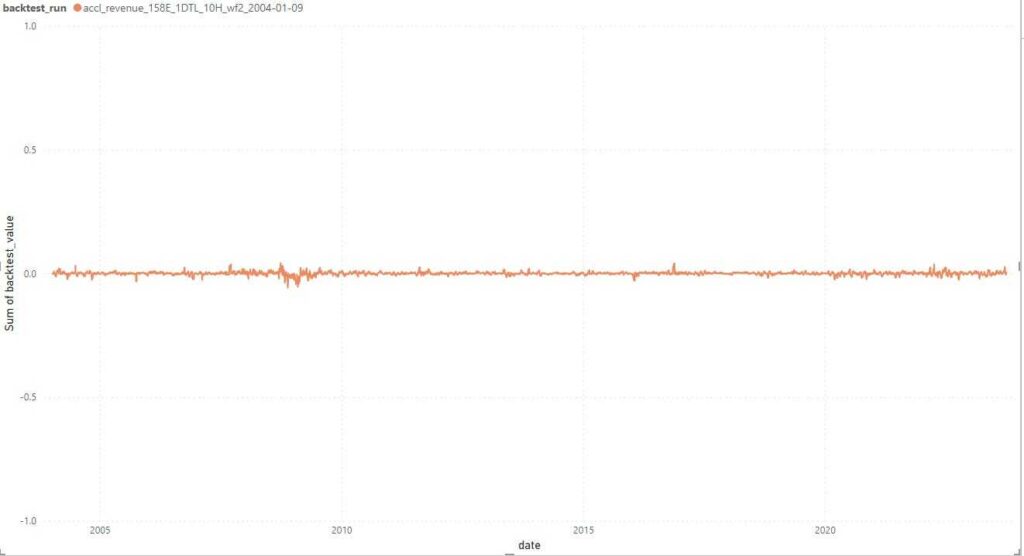
The chart illustrates the cash neutrality of the portfolio – 0 is perfectly cash-neutral.

The second chart is the 6-month rolling correlation between the market and our ACCL portfolio. A perfectly market-neutral portfolio would show a flat line at 0.0 (or no correlation to the market).

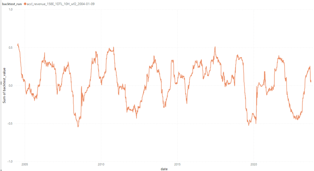
The chart compares the correlation between the ACCL portfolio to the market.

It’s clear from the second chart that we are very much correlated with the market, the correlation at times reaching 50% or so. Moreover, this correlation appears to be cyclical in nature.

How Can We Move Towards Greater Market Neutrality…

A solution to this phenomenon can be implemented via an optimization problem imposed on our portfolio each rebalance period. Many active managers are familiar with the standard optimizations such as “mean-variance” optimization. 

However, in this case, we propose to implement the following optimization problem instead:

Note that h_i is the holding for stock i, β_i is the beta between stock i and the market (estimated in advance according to the CAPM equation above), and h_i,0 is the original holding pre-optimization for stock i.

What this optimization is attempting to do:

• Minimize the squared sum of holdings: the reason for this is that we want to be cash-neutral, and so we want the sum of long$ and short$ to be roughly equal, where shorts are negative so that h_i < 0. In other words, we want the first term above to be as close to zero as possible.
• Minimize the squared sum of the product of beta’s for each stock, times the holdings for that stock: this is the market-neutral constraint. Again, we want the second term above to be as close to zero as possible.
• Finally, as much as possible, reduce the amount of position switching. Since h_i,0 is the original holding for stock i, we impose a cost on changing positions from the original position. We essentially want to tilt things to be market-neutral but minimize the amount we need to change our positioning, thus making the last term as close to zero as possible.

Running this optimization, each rebalance, results in a much improved overall correlation with the market, while still maintaining cash-neutrality as before (nearly a 50% reduction in rolling 6-month market correlation, if we measure the absolute area under the time-series curves in the chart below, where the blue line is the new portfolio). 

You can see that the result isn’t perfect, and this is likely because historical betas aren’t 100% predictive of future betas, something that could be improved on with more advanced techniques like machine learning predictions.

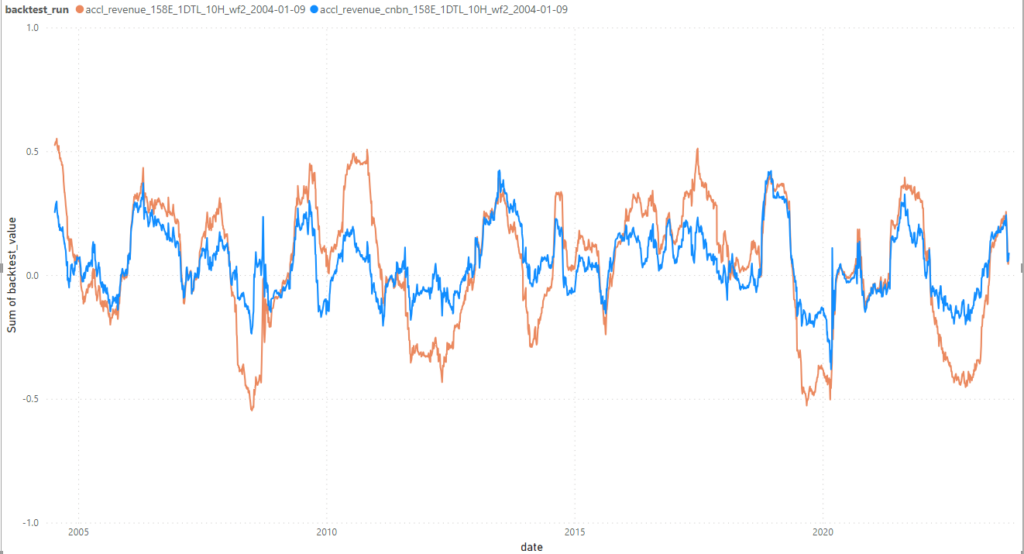
The chart illustrates the correlation between the “market-neutralization” optimization (blue) vs. the cash-neutral strategy (orange).

Finally, we see that the changes in positioning are relatively minor.

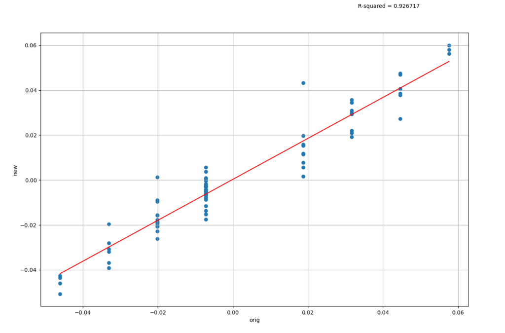
The chart illustrates the changes in position sizes between the market-neutralization (y-axis) and the cash-neutral (x-axis).

In the above scatter, the dots are individual holdings of stocks in the S&P 500 universe on a given rebalance day, where the x-axis is the original pre-market-neutralization, and the y-axis is after the market-neutralization optimization. Notice there is a high R^2 between the position changes indicating very little change in most cases.

A key takeaway here is that we can slightly “nudge” positions without incurring massive trading costs, or shifts in original positioning intent, and achieve a much less market-exposed portfolio.

In Conclusion

At AlphaLayer, we take a multifaceted approach, blending rigorous analysis with innovative strategies to tackle the never-ending challenges/questions that exist in the pursuit of strategies that deliver better risk-adjusted returns.

In this article, we’ve highlighted one way that you can reduce market exposure in actively managed strategies, which provides lower market correlations than a cash-neutral approach.

We continue to explore additional techniques to address the market neutrality issue and many others!

---

1. See Grinold & Khan, Chapter 6, “Fundamental Law of Active Management”, within “Active Portfolio Management” 1995
2. In this experiment, we are only looking at the impact to market correlation and not evaluating a broader set of performance metrics (Sharpe, etc.)
3. Note the holdings are measured in here % portfolio weights, where again, negative weights are short positions

---